Robust detrending examples

Some toy examples to showcase usage for meegkit.detrend module.

Robust referencing is adapted from [1].

References

> [1] de Cheveigné, A., & Arzounian, D. (2018). Robust detrending,

rereferencing, outlier detection, and inpainting for multichannel data. NeuroImage, 172, 903-912.

import matplotlib.pyplot as plt
import numpy as np
from matplotlib.gridspec import GridSpec

from meegkit.detrend import detrend, regress

# import config  # plotting utils

rng = np.random.default_rng(9)

Regression

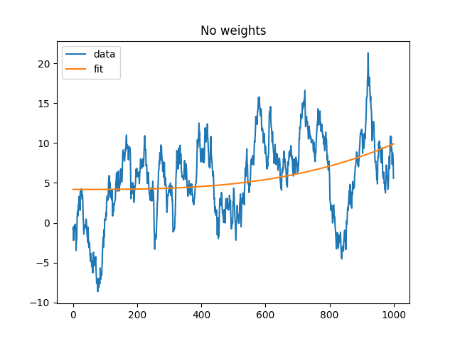
Simple regression example, no weights

We first try to fit a simple random walk process.

x = np.cumsum(rng.standard_normal((1000, 1)), axis=0)
r = np.arange(1000.)[:, None]
r = np.hstack([r, r ** 2, r ** 3])
b, y = regress(x, r)

plt.figure(1)
plt.plot(x, label="data")
plt.plot(y, label="fit")
plt.title("No weights")
plt.legend()
plt.show()

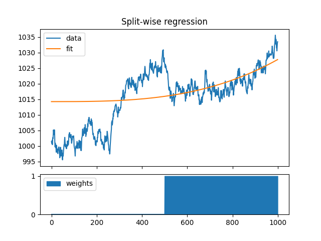
Downweight 1st half of the data

We can also use weights for each time sample. Here we explicitly restrict the fit to the second half of the data by setting weights to zero for the first 500 samples.

x = np.cumsum(rng.standard_normal((1000, 1)), axis=0) + 1000
w = np.ones(y.shape[0])
w[:500] = 0
b, y = regress(x, r, w)

f = plt.figure(3)
gs = GridSpec(4, 1, figure=f)
ax1 = f.add_subplot(gs[:3, 0])
ax1.plot(x, label="data")
ax1.plot(y, label="fit")
ax1.set_xticklabels("")
ax1.set_title("Split-wise regression")
ax1.legend()
ax2 = f.add_subplot(gs[3, 0])
ll, = ax2.plot(np.arange(1000), np.zeros(1000))
ax2.stackplot(np.arange(1000), w, labels=["weights"], color=ll.get_color())
ax2.legend(loc=2)

<matplotlib.legend.Legend object at 0x7fe81ab8cb80>

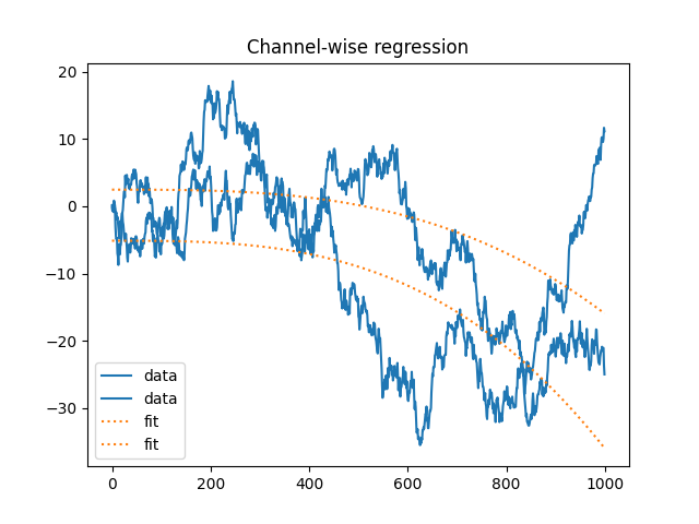
Multichannel regression

x = np.cumsum(rng.standard_normal((1000, 2)), axis=0)
w = np.ones(y.shape[0])
b, y = regress(x, r, w)

plt.figure(4)
plt.plot(x, label="data", color="C0")
plt.plot(y, ls=":", label="fit", color="C1")
plt.title("Channel-wise regression")
plt.legend()

<matplotlib.legend.Legend object at 0x7fe81aa35db0>

Detrending

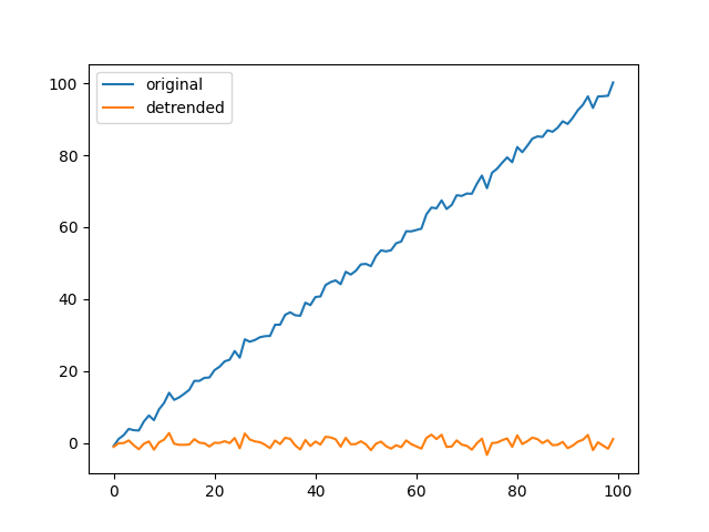
Basic example with a linear trend

x = np.arange(100)[:, None]
x = x + rng.standard_normal(x.shape)
y, _, _ = detrend(x, 1)

plt.figure(5)
plt.plot(x, label="original")
plt.plot(y, label="detrended")
plt.legend()

<matplotlib.legend.Legend object at 0x7fe81aac0fa0>

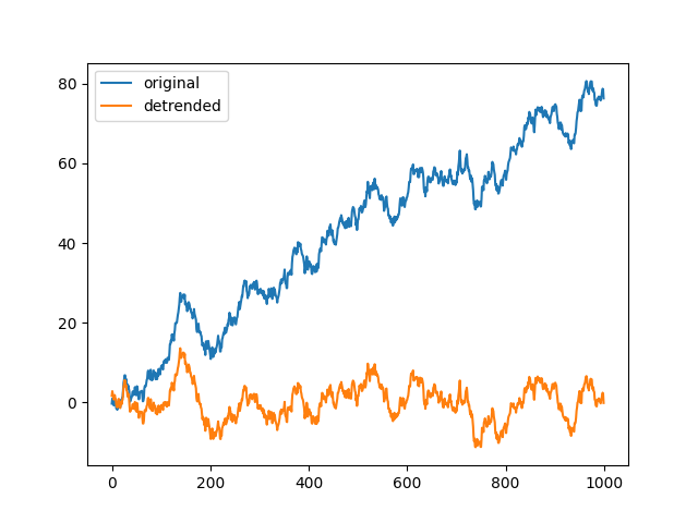
Detrend biased random walk with a third-order polynomial

x = np.cumsum(rng.standard_normal((1000, 1)) + 0.1)
y, _, _ = detrend(x, 3)

plt.figure(6)
plt.plot(x, label="original")
plt.plot(y, label="detrended")
plt.legend()

<matplotlib.legend.Legend object at 0x7fe81a9e7400>

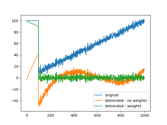
Detrend with weights

Finally, we show how the detrending process handles local artifacts, and how we can advantageously use weights to improve detrending. The raw data consists of gaussian noise with a linear trend, and a storng glitch covering the first 100 timesamples (blue trace). Detrending without weights (orange trace) causes an overestimation of the polynomial order because of the glitch, leading to a mediocre fit. When downweightining this artifactual period, the fit is much improved (green trace).

x = np.linspace(0, 100, 1000)[:, None]
x = x + 3 * rng.standard_normal(x.shape)

# introduce some strong artifact on the first 100 samples
x[:100, :] = 100

# Detrend
y, _, _ = detrend(x, 3, None, threshold=np.inf)

# Same process but this time downweight artifactual window
w = np.ones(x.shape)
w[:100, :] = 0
z, _, _ = detrend(x, 3, w)

plt.figure(7)
plt.plot(x, label="original")
plt.plot(y, label="detrended - no weights")
plt.plot(z, label="detrended - weights")
plt.legend()
plt.show()