DSS example

Find the linear combinations of multichannel data that maximize repeatability over trials.

This example uses synthetic data with a known repeated source, so we can check whether the first DSS component better matches the ground truth than the raw trial average.

Uses meegkit.dss0().

References

[1]

de Cheveigne, A., & Parra, L. C. (2014). Joint decorrelation, a versatile tool for multichannel data analysis. NeuroImage, 98, 487-505.

import matplotlib.pyplot as plt
import numpy as np

from meegkit import dss
from meegkit.utils import fold, rms, tscov, unfold

rng = np.random.default_rng(5)

Create simulated data

# Data are time * channel * trials.
n_samples = 100 * 3
n_chans = 30
n_trials = 100
noise_dim = 20  # dimensionality of noise

# Source signal
source = np.hstack((
    np.zeros((n_samples // 3,)),
    np.sin(2 * np.pi * np.arange(n_samples // 3) / (n_samples / 3)).T,
    np.zeros((n_samples // 3,))))[np.newaxis].T
s = source * rng.standard_normal((1, n_chans))  # 300 * 30
s = s[:, :, np.newaxis]
s = np.tile(s, (1, 1, 100))

# Noise
noise = np.dot(
    unfold(rng.standard_normal((n_samples, noise_dim, n_trials))),
    rng.standard_normal((noise_dim, n_chans)))
noise = fold(noise, n_samples)

# Mix signal and noise
SNR = 0.1
data = noise / rms(noise.flatten()) + SNR * s / rms(s.flatten())

Apply DSS to clean them

# Compute original and biased covariance matrices
c0, _ = tscov(data)

# In this case the biased covariance is simply the covariance of the mean over
# trials
c1, _ = tscov(np.mean(data, 2))

# Apply DSS
[todss, _, pwr0, pwr1] = dss.dss0(c0, c1)
z = fold(np.dot(unfold(data), todss), epoch_size=n_samples)

# Find best components
best_comp = np.mean(z[:, 0, :], -1)
trial_avg_by_channel = np.mean(data, 2)
raw_average = trial_avg_by_channel.mean(axis=1)

# DSS components are sign-indeterminate. Flip to align with the known source
# so the comparison is easier to read.
comp_sign = np.sign(np.corrcoef(source[:, 0], best_comp)[0, 1])
if comp_sign == 0:
    comp_sign = 1.0
best_comp = comp_sign * best_comp

q10, q90 = np.percentile(trial_avg_by_channel, [10, 90], axis=1)
shown_chans = np.linspace(0, n_chans - 1, min(n_chans, 8), dtype=int)

# Compare the recovered component to the known source waveform.
source_corr_raw = np.corrcoef(source[:, 0], raw_average)[0, 1]
source_corr_dss = np.corrcoef(source[:, 0], best_comp)[0, 1]

Plot results

What to look for: - The raw trial average should still be visibly noisy. - The first DSS component should follow the known source more closely. - The reported correlation with the source should improve after DSS.

f, (ax1, ax2, ax3) = plt.subplots(3, 1, figsize=(8, 7), sharex=True,
                                  constrained_layout=True)
time = np.arange(n_samples)
ax1.plot(source, label="source")
ax1.grid(alpha=.2)
ax1.set_ylabel("Amplitude")
ax1.set_title("Ground-truth source")
channel_lines = ax2.plot(time, trial_avg_by_channel[:, shown_chans], color="0.7",
                         lw=.8, alpha=.5)
channel_lines[0].set_label(f"{len(shown_chans)} channels")
for line in channel_lines[1:]:
    line.set_label("_nolegend_")
ax2.plot(time, raw_average, color="C0", lw=2.2, label="channel mean")
ax2.fill_between(time, q10, q90, color="C0", alpha=.18, linewidth=0,
                 label="10-90% range")
ax2.axhline(0, color="0.5", lw=.8, ls=":", zorder=0)
ax2.grid(alpha=.2)
ax2.set_ylabel("Amplitude")
ax2.set_title(f"Trial-averaged observed data (corr = {source_corr_raw:.2f})")
ax3.plot(time, best_comp, label="recovered")
ax3.axhline(0, color="0.5", lw=.8, ls=":", zorder=0)
ax3.grid(alpha=.2)
ax3.set_ylabel("Amplitude")
ax3.set_xlabel("Samples")
ax3.set_title(f"Recovered DSS component (corr = {source_corr_dss:.2f})")
ax1.legend(loc="upper right", fontsize="small")
ax2.legend(loc="upper right", fontsize="small")
ax3.legend(loc="upper right", fontsize="small")
print(f"Correlation with source, raw trial average: {source_corr_raw:.3f}")
print(f"Correlation with source, first DSS component: {source_corr_dss:.3f}")
plt.show()

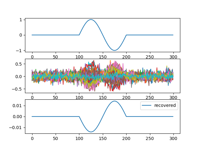
Correlation with source, raw trial average: -0.712
Correlation with source, first DSS component: 1.000