ASR calibration sensitivity

This tutorial-style example illustrates how ASR results depend on the calibration segment used during fitting.

We fit ASR on three candidate calibration windows and compare the resulting channel-wise RMS attenuation. This helps users choose a calibration strategy in real datasets.

The main question is whether the cleaning result is stable across plausible calibration windows, or whether one window yields much stronger attenuation.

Uses meegkit.asr.ASR().

References

[1]

Mullen, T., Kothe, C., Chi, Y., Ojeda, A., Kerth, T., Makeig, S., Jung, T. P., & Cauwenberghs, G. (2015). Real-time neuroimaging and cognitive monitoring using wearable dry EEG. IEEE Transactions on Biomedical Engineering, 62(11), 2553-2567.

import os

import matplotlib.pyplot as plt
import numpy as np

from meegkit.asr import ASR
from meegkit.utils.matrix import sliding_window

raw = np.load(os.path.join("..", "tests", "data", "eeg_raw.npy"))
sfreq = 250

Define candidate calibration windows

In practice, calibration quality strongly affects how aggressively ASR suppresses artifacts. Here we compare three 20-second windows.

windows_sec = {
    "early (0-20s)": (0, 20),
    "middle (10-30s)": (10, 30),
    "late (20-40s)": (20, 40),
}

X = sliding_window(raw, window=int(sfreq), step=int(sfreq))
raw_win = X.reshape(raw.shape[0], -1)
rms_before = np.sqrt(np.mean(raw_win ** 2, axis=1))

ratios = {}

Fit and apply ASR for each candidate window

for label, (start_s, stop_s) in windows_sec.items():
    train_idx = np.arange(start_s * sfreq, stop_s * sfreq, dtype=int)

    asr = ASR(method="euclid")
    asr.fit(raw[:, train_idx])

    Y = np.zeros_like(X)
    for i in range(X.shape[1]):
        Y[:, i, :] = asr.transform(X[:, i, :])

    clean = Y.reshape(raw.shape[0], -1)
    rms_after = np.sqrt(np.mean(clean ** 2, axis=1))
    ratios[label] = rms_after / np.maximum(rms_before, np.finfo(float).eps)

Visualize channel-wise attenuation by calibration choice

What to look for: - Ratios below 1 indicate attenuation. - Large differences across windows suggest sensitivity to calibration period.

fig, ax = plt.subplots(1, 1, figsize=(8, 4))
channels = np.arange(raw.shape[0])

for label, ratio in ratios.items():
    ax.plot(channels, ratio, "o-", lw=1.5, label=label)

ax.axhline(1.0, color="k", ls=":", lw=1)
ax.set_xticks(channels)
ax.set_xlabel("Channel")
ax.set_ylabel("RMS ratio (after / before)")
ax.set_title("ASR sensitivity to calibration window")
ax.grid(True, axis="y", ls=":", alpha=.4)
ax.legend(fontsize="small")
plt.tight_layout()

for label, ratio in ratios.items():
    print(f"{label:>16}: median ratio = {np.median(ratio):.3f}")

best_label = min(ratios, key=lambda key: np.median(ratios[key]))
print(f"Most aggressive calibration in this example: {best_label}")
print("Interpretation: large separation between curves means the ASR result")
print("depends strongly on which segment is treated as clean calibration data.")

plt.show()

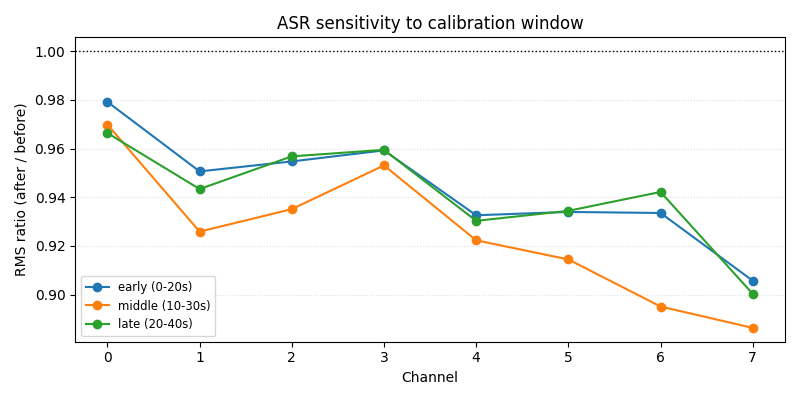
   early (0-20s): median ratio = 0.942
 middle (10-30s): median ratio = 0.924
   late (20-40s): median ratio = 0.943
Most aggressive calibration in this example: middle (10-30s)
Interpretation: large separation between curves means the ASR result
depends strongly on which segment is treated as clean calibration data.